Background on Gradients

Implicit Function Theorem

An implicit function, $r : \mathbf{R}^{n_w} \times \mathbf{R}^{n_\theta} \rightarrow \mathbf{R}^{n_w}$, is defined as

\[r(w^*; \theta) = 0,\]

for solution $w^* \in \mathbf{R}^{n_w}$ and problem data $\theta \in \mathbf{R}^{n_\theta}$. At a solution point of the above equation the sensitivities of the solution with respect to the problem data, i.e., $\partial w^* / \partial \theta$, can be computed under certain conditions. First, we approximate the above equation to first order:

\[ \frac{\partial r}{\partial w} \delta w + \frac{\partial r}{\partial \theta} \delta \theta = 0,\]

and then solve for the relationship:

\[\frac{\partial w^*}{\partial \theta} = -\Big(\frac{\partial r}{\partial w}\Big)^{-1} \frac{\partial r}{\partial \theta}. \quad \quad(1)\]

In case $(\partial r / \partial w)^{-1}$ is not well defined, (e.g., not full rank) we can either apply regularization or approximately solve (1) with, for example, a least-squares approach.

Often, Newton's method is employed to find solutions to the implicit equation and custom linear-system solvers can efficiently compute search directions for this purpose. Importantly, the factorization of $\partial r / \partial w$ used to find a solution can be reused to compute (1) at very low computational cost using only back-substitution. Additionally, each element of the problem-data sensitivity can be computed in parallel.

Dojo's Gradient

At a solution point, $w^*(\theta, \kappa)$, the sensitivity of the solution with respect to the problem data, i.e., $\partial w^* / \partial \theta$, is efficiently computed using the implicit-function theorem (1) to differentiate through the solver's residual.

The efficient linear-system solver used for the simulator, as well as the computation and factorization of $\partial r / \partial w$, is used to compute the sensitivities for each element of the problem data. Calculations over the individual columns of $\partial r / \partial \theta$ can be performed in parallel.

The problem data for each simulation step include: the previous and current configurations, control input, and additional terms like the time step, friction coefficients, and parameters of each body. The chain rule is utilized to compute gradients with respect to the finite-difference velocities as well as transformations between minimal- and maximal-coordinate representations.

In many robotics scenarios, we are interested in gradient information through contact events. Instead of computing gradients for hard contact with zero or very small central-path parameters, we use a relaxed value from intermediate solutions $w^*(\theta, \kappa > 0)$ corresponding to a soft contact model. In practice, we find that these smooth gradients greatly improve the performance of gradient-based optimization methods.

Gradient Comparison

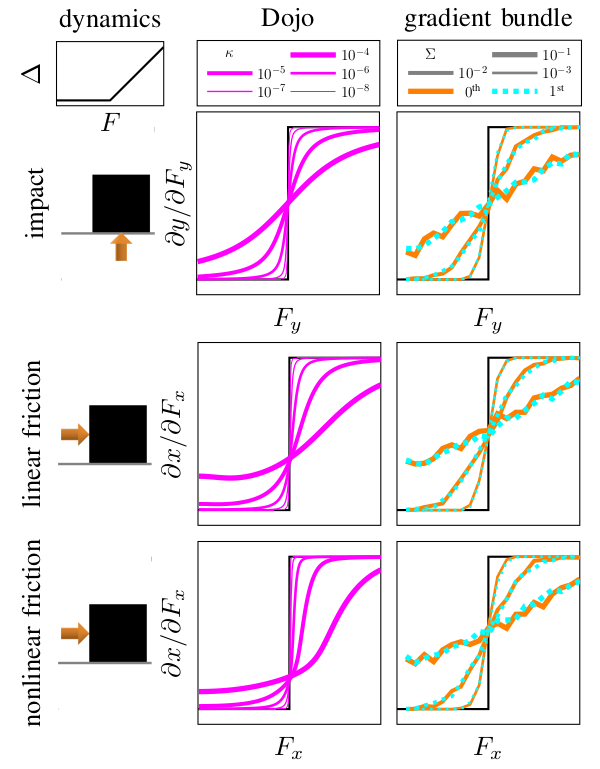
Gradient comparison between randomized smoothing and Dojo's smooth gradients. The dynamics for a box in the $XY$ plane that is resting on a flat surface and displaced an amount $\Delta$ by an input $F$ (top left). Its corresponding exact gradients are shown in black. Gradient bundles (right column) are computed using sampling schemes with varying covariances $\Sigma$ and $500$ samples. Dojo's gradients (middle column) are computed for different values of $\kappa$, corresponding to the smoothness of the contact model. Compared to the 500-sample gradient bundle, Dojo's gradients are not noisy and are a 100 times faster to compute with a single worker.