System Identification

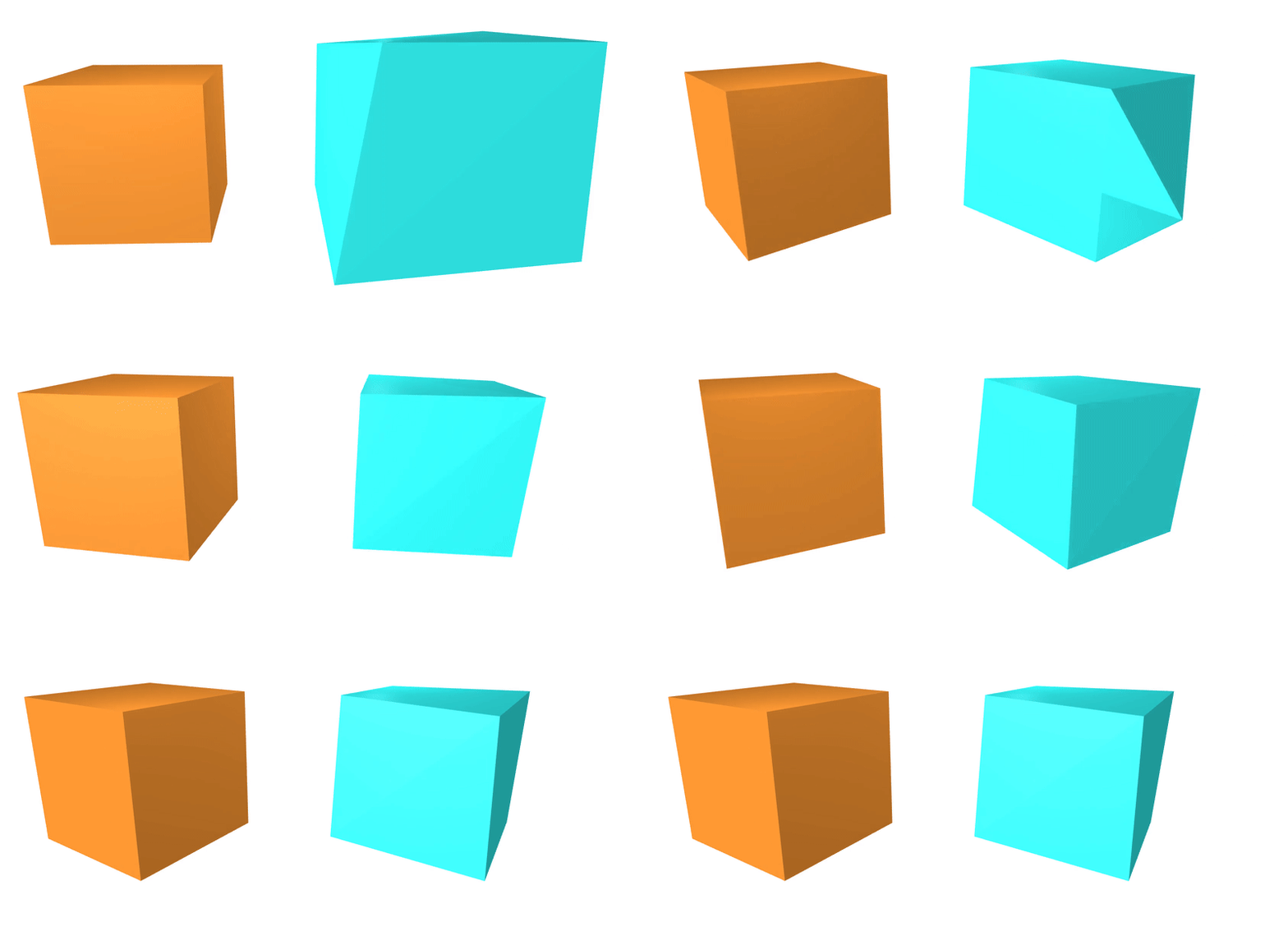
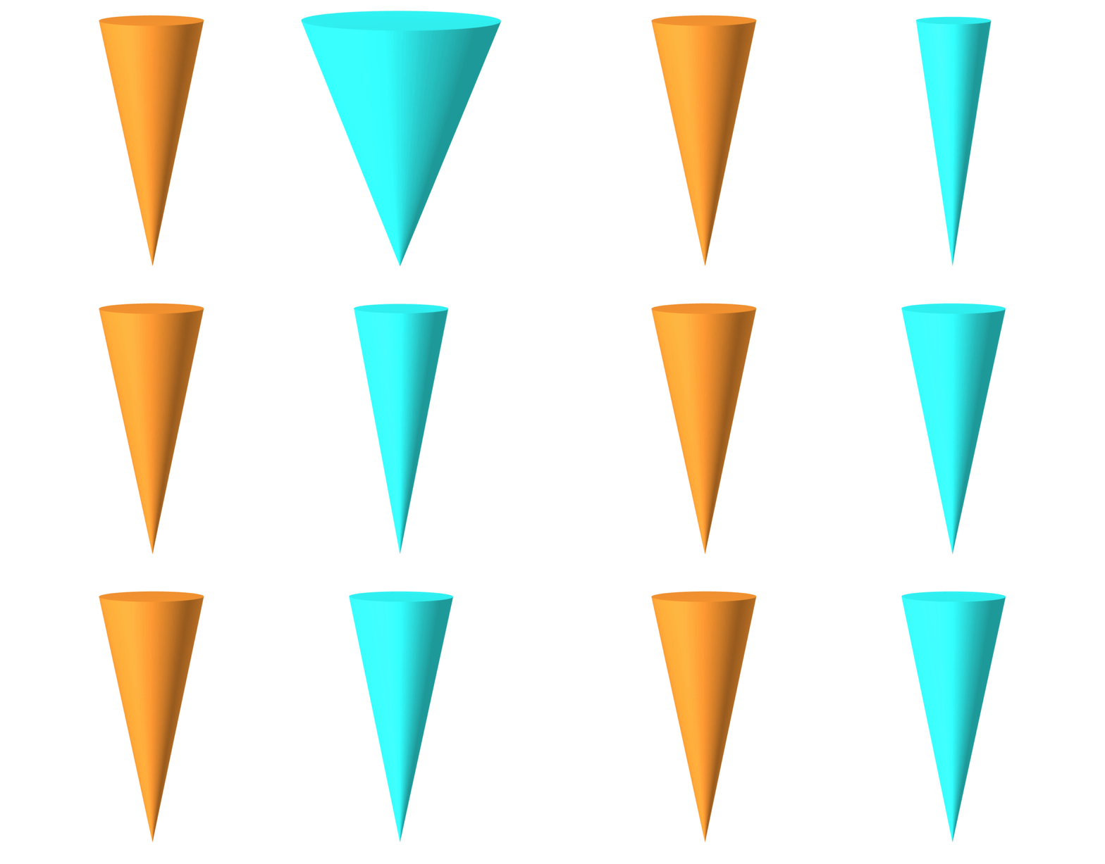
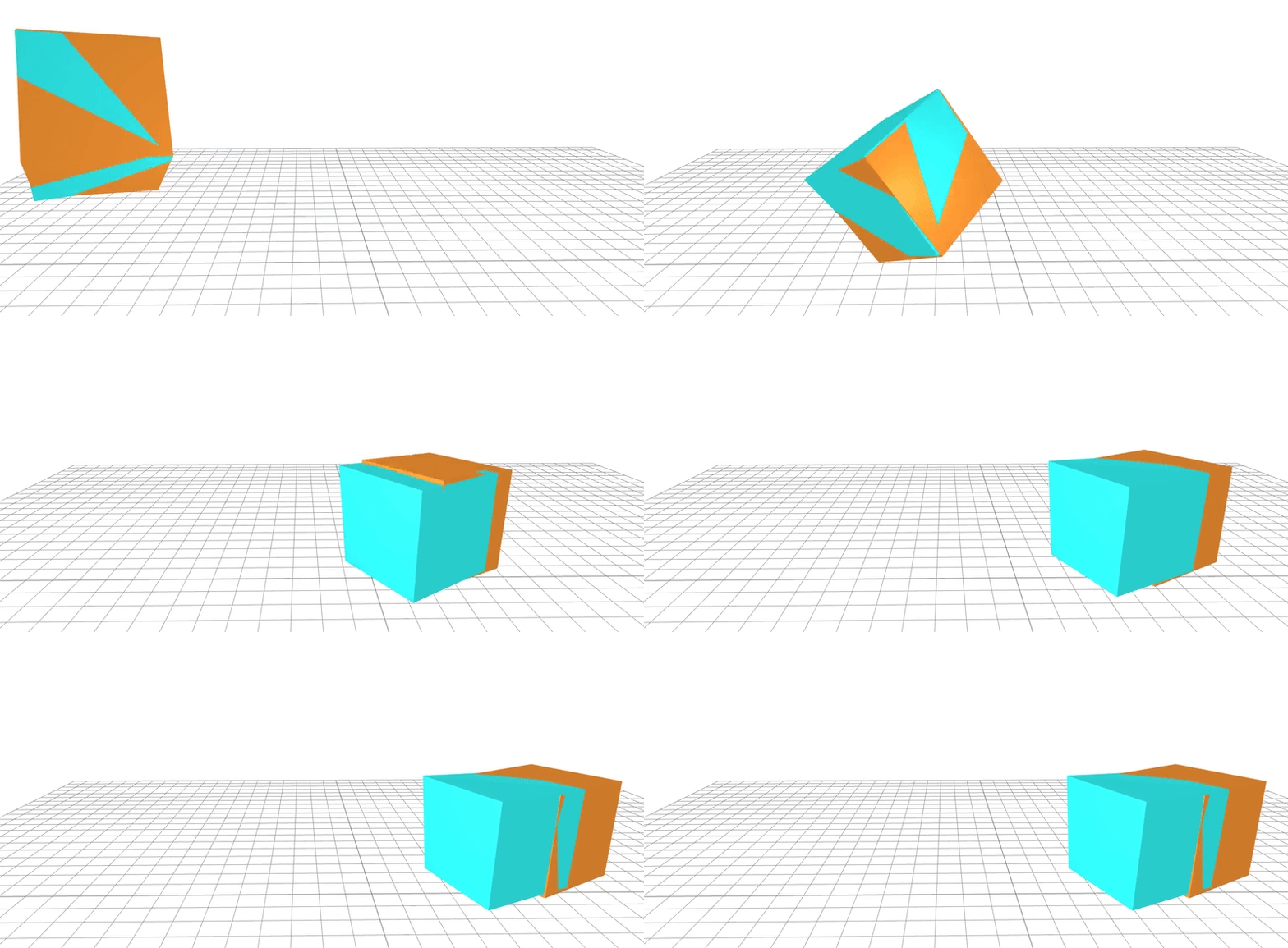
A real-world dataset is used to learn the geometric and friction properties of a block being tossed onto a flat surface. Gradient-based optimization is employed to regress parameters and real-to-sim validation is performed. The ground truth system is shown in orange and the learned system in blue.

Geometry

The eight locations of the block's corners relative to its center of mass are learned.

Friction

A friction coefficient, describing a friction cone, is learned for all of the contact points.

Real-To-Sim

The system parameters are learned to within a $\pm 5 \%$ error from their ground-truth values. These parameters are then compared to the ground-truth system in simulation.

Learning

The cost function:

$\mathcal{L}(\mathcal{D}, \theta) = \sum_{Z \in \mathcal{D}} L(Z, \theta) = \sum_{Z \in \mathcal{D}} \frac{1}{2} ||s(z_{-}, z, \theta) - z_{+}||_W^2$,

is used where $\mathcal{D}$ is a dataset of trajectories containing tuples $(z_{-}, z, z_{+})$ of state sequences, with system parameters $\theta \in \mathbf{R}^p$, and where $s : \mathbf{Z} \times \mathbf{Z} \times \mathbf{R}^p \rightarrow \mathbf{Z}$ represents the simulator.

A quasi-Newton method is employed to optimize the cost function and uses gradients:

$\frac{\partial L}{\partial \theta} = {\frac{\partial s}{\partial \theta}}^T W \Big(s(z_{-}, z, \theta) - z_{+} \Big)$,

and the following Gauss-Newton approximation:

$\frac{\partial^2 L}{\partial \theta^2} \approx {\frac{\partial s}{\partial \theta}}^T W \frac{\partial s}{\partial \theta}$,

of the cost function Hessian, which only relies on Jacobians from Dojo.